Force Matching#
Force matching is a bottom-up method to derive coarse-grained potentials $U_\theta$ from atomistic reference data. In a variational formulation, the approach learns a set of parameters $\theta$ by optimizing the error $\chi^2$ of predicted coarse forces $\mathbf F_I^\theta(\mathbf R)$ on the coarse-grained sites $\mathbf R = M(\mathbf r)$ [1]
Load Data#
In this example, we use reference data from an all-atomistic simulation of ethane. We obtained this data in the example Prior Simulation.

train_ratio = 0.5

box = jnp.asarray([1.0, 1.0, 1.0])

all_forces = preprocessing.get_dataset(base_path / "forces_ethane.npy")
all_positions = preprocessing.get_dataset(base_path / "positions_ethane.npy")
Compute Mapping#
The reference data contains only fine-grained forces $\mathbf f_i$ and positions $\mathbf r_i$. Thus, we must define a mapping $M$ that derives the positions of the coarse-grained sites $\mathcal I_I$ and the forces acting on them [1]
We select the two carbon atoms $C_1$ and $C_2$ as locations of the coarse-grained sites $\mathcal I_1$ and $\mathcal I_2$ and neglect the hydrogen atoms. We then compute the effective coarse-grained forces from the atomistic forces via the corresponding linear mapping [1]
# Center of Mass (COM) mapping
displacement_fn, shift_fn = space.periodic_general(box, fractional_coordinates=True)

# Scale the position data into fractional coordinates
position_dataset = preprocessing.scale_dataset_fractional(all_positions, box)

masses = jnp.asarray([15.035, 1.011, 1.011, 1.011])

weights = jnp.asarray([
    [1, 0.0000, 0, 0, 0, 0.000, 0.000, 0.000],
    [0.0000, 1, 0.000, 0.000, 0.000, 0, 0, 0]
])

position_dataset, force_dataset = preprocessing.map_dataset(
    position_dataset, displacement_fn, shift_fn, weights, weights, all_forces
)
Setup Model#
As a coarse-grained potential model, we choose a simple spring bond
To ensure that the model parameters remain positive during optimization, we transform them into a constraint space $\theta_1 = \log b_0,\ \theta_2= \log k_B$.
r_init = position_dataset[0, ...]

displacement_fn, shift_fn = space.periodic_general(box, fractional_coordinates=True)
neighbor_fn = custom_partition.masked_neighbor_list(displacement_fn, r_cutoff=1.0)

nbrs_init = neighbor_fn.allocate(r_init)

init_params = {
    "log_b0": jnp.log(0.11),
    "log_kb": jnp.log(5000.0)
}

def energy_fn_template(energy_params):
    harmonic_energy_fn = energy.simple_spring_bond(
        displacement_fn, bond=jnp.asarray([[0, 1]]),
        length=jnp.exp(energy_params["log_b0"]),
        epsilon=jnp.exp(energy_params["log_kb"]),
        alpha=2.0
    )

    return harmonic_energy_fn

def force_fn_template(energy_params):
    neg_energy_fn = lambda r, **kwargs: -energy_fn_template(energy_params)(r, **kwargs)
    return jax.grad(neg_energy_fn, argnums=0)

@jax.value_and_grad
def test_loss_fn(params, r, f):
    return jnp.mean(jnp.sum((f - force_fn_template(params)(r, neighbor=nbrs_init)) ** 2, axis=-1))

sample_idx = 0

print(f"Energy with initial params is {energy_fn_template(init_params)(position_dataset[sample_idx, ...], neighbor=nbrs_init)}")
print(f"Forces with initial params are\n{force_fn_template(init_params)(position_dataset[sample_idx, ...], neighbor=nbrs_init)}")
print(f"Parameter gradients on initial sample are\n{test_loss_fn(init_params, position_dataset[sample_idx, ...], force_dataset[sample_idx, ...])[1]}")
/home/docs/checkouts/readthedocs.org/user_builds/chemtrain/envs/latest/lib/python3.11/site-packages/jax/_src/numpy/reductions.py:230: UserWarning: Explicitly requested dtype <class 'jax.numpy.float64'> requested in sum is not available, and will be truncated to dtype float32. To enable more dtypes, set the jax_enable_x64 configuration option or the JAX_ENABLE_X64 shell environment variable. See https://github.com/jax-ml/jax#current-gotchas for more.
  return _reduction(a, "sum", lax.add, 0, preproc=_cast_to_numeric,
Energy with initial params is 2.144806146621704
Forces with initial params are
[[-112.5239    -50.379333  -79.04647 ]
 [ 112.5239     50.379333   79.04647 ]]
Parameter gradients on initial sample are
{'log_b0': Array(-71939.1, dtype=float32, weak_type=True), 'log_kb': Array(19155.629, dtype=float32, weak_type=True)}
Analytical Solution#
As our model relies only on the magnitude of the displacement between $C_1$ and $C_2$, we compute this distance and plot it.
disp = jax.vmap(displacement_fn)(position_dataset[:, 0, :], position_dataset[:, 1, :])
dist_CC = jnp.sqrt(jnp.sum(disp ** 2, axis=-1))

plt.figure()
plt.hist(dist_CC, bins=100)
plt.xlabel("Distance C_1 - C_2 [nm]")
plt.ylabel("Count")
Text(0, 0.5, 'Count')
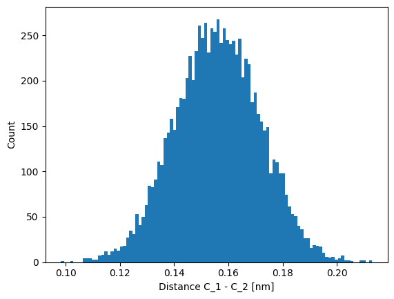
Indeed, the distance between the two carbon atoms is approximately Gaussian distributed. Hence, the choice of a harmonic potential model is reasonable.
However, we want to check whether our force data supports this hypothesis. Therefore, we project the forces onto the displacement vector between the two carbon atoms.
disp_dir = disp / dist_CC[:, None]
force_proj = jnp.einsum('ijk, i...k->ij', force_dataset, disp_dir)

plt.figure()
plt.scatter(dist_CC, force_proj[:, 0], color="r", s=1)
plt.scatter(dist_CC, force_proj[:, 1], color="b", s=1)
plt.xlabel("Distance C_1 - C_2 [nm]")
plt.ylabel("Projected Force")
Text(0, 0.5, 'Projected Force')
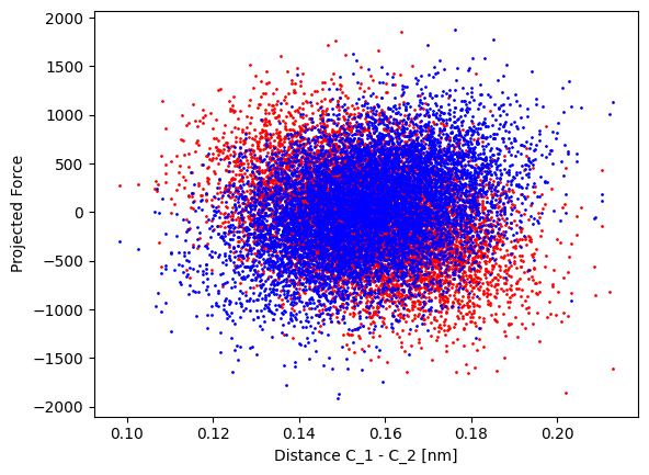
We see that also the force reference data is quite noisy, but still correlates with the distance between the coarse-grained sites.
Since this relationship is linear, we might estimate the parameters of the model via a linear regression fit.
# Least squares solution
lhs = jnp.stack((dist_CC, jnp.ones_like(dist_CC)), axis=-1)
rhs = -force_proj[:, (0,)]

kb, c = jnp.linalg.lstsq(lhs, rhs, rcond=None)[0]
b0 = -c / kb

print(f"Estimated potential parameters are {kb[0] :.1f} kJ/mol/nm^2 and {b0[0] :.3f} nm")
Estimated potential parameters are 10072.9 kJ/mol/nm^2 and 0.153 nm
Setup Optimizer#
subsample = 25
batch_per_device = 10
epochs = 20
initial_lr = 0.02
lr_decay = 0.05

lrd = int(position_dataset.shape[0] / subsample / batch_per_device * epochs)
lr_schedule = optax.exponential_decay(initial_lr, lrd, lr_decay)
optimizer = optax.chain(
    optax.scale_by_adam(0.9, 0.95),
    optax.scale_by_schedule(lr_schedule),
    # Flips the sign of the update for gradient descend
    optax.scale_by_learning_rate(1.0),
)
Setup Force Matching#
force_matching = ForceMatching(
    init_params=init_params, energy_fn_template=energy_fn_template,
    nbrs_init=nbrs_init, optimizer=optimizer, batch_per_device=batch_per_device,
)

# We can provide numpy arrays to initialize the datasets for training,
# validation, and testing in a single step
force_matching.set_datasets({
    "F": force_dataset[::subsample, :, :],
    "R": position_dataset[::subsample, :, :],
}, train_ratio=train_ratio)
force_matching.train(epochs, checkpoint_freq=1000)
# We can also provide completely new samples for a single stage, e.g., testing
force_matching.set_dataset({
    "F": force_dataset[1::subsample, :, :],
    "R": position_dataset[1::subsample, :, :],
}, stage = "testing")

mae_error = force_matching.evaluate_mae_testset()
print(mae_error)
Always recompute the neighbor list!
[Force] Found precomputed forces.
F: MAE = 419.0875
None
Results#
plt.plot(force_matching.train_losses)
plt.xticks(ticks=range(0, epochs + 1, 5))
plt.xlabel("Epoch")
plt.ylabel("Force Error")
Text(0, 0.5, 'Force Error')
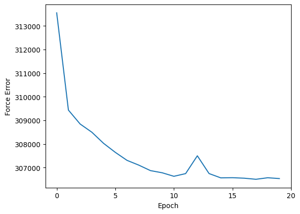
Finally, we compare the values obtained from a least-squares fit to those obtained from force-matching.
pred_parameters = tree_util.tree_map(jnp.exp, force_matching.params)

b0_err = jnp.abs(b0[0] - pred_parameters["log_b0"])
kb_err = jnp.abs(kb[0] - pred_parameters["log_kb"])

print(f"Force matching predicted {pred_parameters['log_b0']:.3f} nm and {pred_parameters['log_kb']:.1f} kJ/mol/nm^2")
print(f"Least squares predicted {b0[0]:.3f} nm and {kb[0]:.1f} kJ/mol/nm^2")
print(f"Absolute error in b0 is {b0_err:.3f} nm and in kb is {kb_err:.1f} kJ/mol/nm^2")
Force matching predicted 0.152 nm and 9550.4 kJ/mol/nm^2
Least squares predicted 0.153 nm and 10072.9 kJ/mol/nm^2
Absolute error in b0 is 0.001 nm and in kb is 522.5 kJ/mol/nm^2
Further Reading#
Examples#
Publications#
Stephan Thaler, Maximilian Stupp, Julija Zavadlav; Deep coarse-grained potentials via relative entropy minimization. J. Chem. Phys. 28 December 2022; 157 (24): 244103. https://doi.org/10.1063/5.0124538