Relative Entropy Minimization#
Principle of Relative Entropy#
Relative entropy provides a fundamental link between models of different scales [1]. Measuring the loss of information induced by the coarse-graining [2], it is thus a desirable objective to minimize.
For a corase-grained model $p^\text{CG}_\theta(\mathbf R)$ on coarse-grained sites $\mathbf R$ connected to the sites of a fine-scale model $p^\text{AA}(\mathbf r)$ via a mapping $\mathbf R = M(\mathbf r)$, the relative entropy is [2]
$$ S_\text{rel} = S_\text{map} + \int p^\text{AA}(\mathbf r)\log \frac{p^\text{AA}(\mathbf r)}{p^\text{CG}(M(\mathbf r))}d\mathbf r. $$
For a canonical ensemble $p(\mathbf r) \propto e^{-\beta U(\mathbf r)}$ at temperature $T = \frac{1}{k_B \beta}$, the relative entropy further decomposes to
$$ S_\text{rel} = S_\text{map} + \beta \left\langle U_\theta^\text{CG}(M(\mathbf r)) - U^\text{AA}(\mathbf r)\right\rangle_\text{AA} - \beta(A_\theta^\text{CG} - A^\text{AA}). $$
The first part $S_\text{rel}$ measures the unavoidable loss of information due to the degeneracy of the mapping. This part is, however, independent of the fine-grained and coarse-grained distributions.
The second part is the expected difference between the predicted potential energies $U_\theta^\text{CG}(M(\mathbf r)) - U^\text{AA}(\mathbf r)$ in the fine-scaled ensemble. This part is simple to estimate. Analogous to force-matching, the estimation involves pre-computing an atomistic trajectory, followed by a batched gradient-based optimization.
The last part is the free energy difference between the fine-scaled and coarse-grained ensembles. Since the free energy normalizes a distribution
$$ A_\theta = -\frac{1}{\beta}\log \int e^{-\beta U_\theta}dx, $$ it is not a quantity directly predictable from individual samples of the potential energy model. However, several routines exist to estimate the difference of free energies $A_\theta^\text{CG} = \Delta A_\theta^\text{CG} + \tilde A^\text{CG}$ to a reference potential $\tilde U^\text{CG}$.
Thus, the exact computation of the relative entropy is infeasible. Nevertheless, we can collect all terms directly depending on $\theta$ in a new objective
$$ \mathcal L_\text{RE}(\theta) = \beta\left(\left\langle U_\theta^\text{CG}(M(R))\right\rangle_\text{AA} - \Delta A_\theta^\text{CG}\right). $$
This objective has precisely the same gradients as the relative entropy
$$ \frac{\partial}{\partial \theta} \mathcal L(\theta) = \frac{\partial}{\partial \theta}S_\text{rel}. $$
Unfortunately, the objective is no longer lower bound by $0$, reached by the relative entropy under perfect preservation of information. Nevertheless, chemtrain enables the estimation of all the contributions to the loss. Thus, chemtrain can compute the correct gradients via algorithmic differentiation and enable training via the Relative Entropy objective.
Load Data#
This example follows the Force Matching guide. Again, we use reference data from an all-atomistic simulation of ethane. We obtained this data in the example Prior Simulation.

train_ratio = 0.5

box = jnp.asarray([1.0, 1.0, 1.0])
kT = 2.56

all_forces = preprocessing.get_dataset(base_path / "forces_ethane.npy")
all_positions = preprocessing.get_dataset(base_path / "positions_ethane.npy")
Compute Mapping#
The reference data contains only fine-grained forces $\mathbf f_i$ and positions $\mathbf r_i$. Thus, we must define a mapping $M$ that derives the positions of the coarse-grained sites $\mathcal I_I$ [3]
We select the two carbon atoms $C_1$ and $C_2$ as locations of the coarse-grained sites $\mathcal I_1$ and $\mathcal I_2$ and neglect the hydrogen atoms.
# Heacy-atoms mapping
displacement_fn, shift_fn = space.periodic_general(box, fractional_coordinates=True)

# Scale the position data into fractional coordinates
position_dataset = preprocessing.scale_dataset_fractional(all_positions, box)

masses = jnp.asarray([15.035, 1.011, 1.011, 1.011])

weights = jnp.asarray([
    [1, 0.0000, 0, 0, 0, 0.000, 0.000, 0.000],
    [0.0000, 1, 0.000, 0.000, 0.000, 0, 0, 0]
])

position_dataset = preprocessing.map_dataset(
    position_dataset, displacement_fn, shift_fn, weights,
)
Setup Model#
As a coarse-grained potential model, we choose a simple spring bond
To ensure that the model parameters remain positive during optimization, we transform them into a constraint space $\theta_1 = \log b_0,\ \theta_2= \log k_b$.
r_init = position_dataset[0, ...]

displacement_fn, shift_fn = space.periodic_general(box, fractional_coordinates=True)
neighbor_fn = partition.neighbor_list(
    displacement_fn, box, 1.0, fractional_coordinates=True, disable_cell_list=True)

nbrs_init = neighbor_fn.allocate(r_init)

init_params = {
    "log_b0": jnp.log(0.11),
    "log_kb": jnp.log(1000.0)
}

def energy_fn_template(energy_params):
    harmonic_energy_fn = energy.simple_spring_bond(
        displacement_fn, bond=jnp.asarray([[0, 1]]),
        length=jnp.exp(energy_params["log_b0"]),
        epsilon=jnp.exp(energy_params["log_kb"]),
        alpha=2.0
    )

    return harmonic_energy_fn

sample_idx = 0

print(f"Energy with initial params is {energy_fn_template(init_params)(position_dataset[sample_idx, ...], neighbor=nbrs_init)}")
Energy with initial params is 1.105982780456543
/home/docs/checkouts/readthedocs.org/user_builds/chemtrain/envs/latest/lib/python3.11/site-packages/jax/_src/numpy/reductions.py:230: UserWarning: Explicitly requested dtype <class 'jax.numpy.float64'> requested in sum is not available, and will be truncated to dtype float32. To enable more dtypes, set the jax_enable_x64 configuration option or the JAX_ENABLE_X64 shell environment variable. See https://github.com/jax-ml/jax#current-gotchas for more.
  return _reduction(a, "sum", lax.add, 0, preproc=_cast_to_numeric,
Analytical Solution#
As our model relies only on the magnitude of the displacement between $C_1$ and $C_2$, we compute this distance and plot it.
disp = jax.vmap(displacement_fn)(position_dataset[:, 0, :], position_dataset[:, 1, :])
dist_CC = jnp.sqrt(jnp.sum(disp ** 2, axis=-1))

plt.figure()
plt.hist(dist_CC, bins=100)
plt.xlabel("Distance C_1 - C_2 [nm]")
plt.ylabel("Count")
Text(0, 0.5, 'Count')
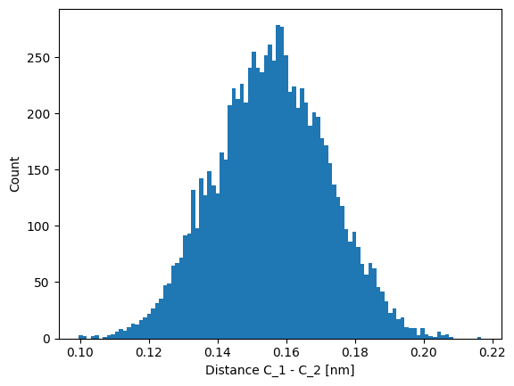
Indeed, the distance between the two carbon atoms is approximately Gaussian distributed. Hence, the choice of a harmonic potential model is reasonable.
Thus, we might estimate the parameters of the model by computing the mean and variance of the particle distance.
$$ b_0 = \mathbb E[|\mathbf R_1 - \mathbf R_2|], \quad k_b = \frac{1}{\beta \operatorname{Var}[|\mathbf R_1 - \mathbf R_2|]} $$
# Analytical solution
b0 = jnp.mean(dist_CC)
kb = kT / jnp.var(dist_CC)

print(f"Estimated potential parameters are {kb :.1f} kJ/mol/nm^2 and {b0 :.3f} nm")
Estimated potential parameters are 9598.2 kJ/mol/nm^2 and 0.156 nm
Setup Optimizer#
epochs = 100
initial_lr = 0.5
lr_decay = 0.1

lrd = int(position_dataset.shape[0] / epochs)
lr_schedule = optax.exponential_decay(initial_lr, lrd, lr_decay)
optimizer = optax.chain(
    optax.scale_by_adam(),
    optax.scale_by_schedule(lr_schedule),
    # Flips the sign of the update for gradient descend
    optax.scale_by_learning_rate(1.0),
)
Setup Simulator#
timings = ensemble.sampling.process_printouts(
    time_step=0.002, total_time=1e3, t_equilib=1e2,
    print_every=0.1, t_start=0.0
)

init_ref_state, sim_template = ensemble.sampling.initialize_simulator_template(
    simulate.nvt_langevin, shift_fn=shift_fn, nbrs=nbrs_init,
    init_with_PRNGKey=True, extra_simulator_kwargs={"kT": kT, "gamma": 1.0, "dt": 0.002}
)

cg_masses = masses[0]

reference_state = init_ref_state(
    random.PRNGKey(11), r_init,
    energy_or_force_fn=energy_fn_template(init_params),
    init_sim_kwargs={"mass": cg_masses, "neighbor": nbrs_init}
)
Setup Relative Entropy Minimization#
relative_entropy = RelativeEntropy(
    init_params=init_params, optimizer=optimizer,
    reweight_ratio=1.1, sim_batch_size=1,
    energy_fn_template=energy_fn_template,
)

subsampled_dataset = position_dataset[::100, ...]
print(f"Dataset has shape {subsampled_dataset.shape}")

relative_entropy.add_statepoint(
    position_dataset, energy_fn_template,
    sim_template, neighbor_fn, timings,
    {'kT': kT}, reference_state,
)

relative_entropy.init_step_size_adaption(0.1)
relative_entropy.train(epochs)
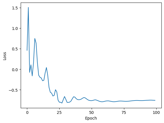
Results#
plt.figure()
plt.plot(relative_entropy.delta_re[0])
plt.xticks(ticks=range(0, epochs + 1, 25))
plt.xlabel("Epoch")
plt.ylabel("Loss")
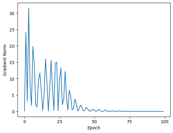
plt.figure()
plt.plot(relative_entropy.gradient_norm_history)
plt.xticks(ticks=range(0, epochs + 1, 25))
plt.xlabel("Epoch")
plt.ylabel("Gradient Norm")
Text(0, 0.5, 'Gradient Norm')
Finally, we compare the values obtained from a Gaussian fit to those obtained from relative entropy minimization.
pred_parameters = tree_util.tree_map(jnp.exp, relative_entropy.params)

b0_err = jnp.abs(b0 - pred_parameters["log_b0"])
kb_err = jnp.abs(kb - pred_parameters["log_kb"])

print(f"RE min. predicted {pred_parameters['log_b0']:.3f} nm and {pred_parameters['log_kb']:.1f} kJ/mol/nm^2")
print(f"Gaussian fit predicted {b0:.3f} nm and {kb:.1f} kJ/mol/nm^2")
print(f"Absolute error in b0 is {b0_err:.3f} nm and in kb is {kb_err:.1f} kJ/mol/nm^2")
RE min. predicted 0.152 nm and 9245.5 kJ/mol/nm^2
Gaussian fit predicted 0.156 nm and 9598.2 kJ/mol/nm^2
Absolute error in b0 is 0.004 nm and in kb is 352.7 kJ/mol/nm^2
Further Reading#
Examples#
Publications#
Stephan Thaler, Maximilian Stupp, Julija Zavadlav; Deep coarse-grained potentials via relative entropy minimization. J. Chem. Phys. 28 December 2022; 157 (24): 244103. https://doi.org/10.1063/5.0124538